Automatic Relevance Determination for Functional Data Representation

…a Vignette on Functional Data Analysis

An approach to functional data representation based on automatic relevance determination.
Author
Published

July 10, 2025

Last updated 2025/07/10.

Introduction

Data

For this particular study, we consider two distinct data sets, the Motorcycle data set and the Canadian weather data set: the former is frequently studied in the overall spline smoothing context (as well as overall studies in Nonparametric Statistics), whilst the latter is most often used in the specific context of Functional Data Analysis. We will also present a brief simulation study. The R chunk provided below loads the relevant packages utilized throughout.

Show R code
library("tidyverse")  ## R package for tidy data manipulation and visualization
library("extrafont")  ## R package for using nice fonts in figures
library("fda")        ## R package for functional data analysis
library("MASS")
library("magrittr")   ## R package for pipes
library("patchwork")  ## R package for plot composition
library("reshape2")
library("rstan")

The Motorcycle data set

The Motorcycle data set (seen in Silverman (1985), and available in the R programming language in the package MASS) consists of \(n = 133\) measurements obtained through an experiment which simulated motorcycle accidents with the goal of determining the efficacy of crash helmets: an accelerometer was fitted to an object which was later submitted to repeated mechanical impacts, and the resulting acceleration was measured in the instants subsequent to the impacts. We denote the measurements of the time (in milliseconds) elapsed since the impact occurs as \(t_j\), and the acceleration (in g) measured at the corresponding instant as \(y_j\), hence we denote the full data set as \(\{t_j, y_j\}^n_{j = 1}\). Some observations can be made with respect to the set of instants \(\{t_j\}^n_{j = 1}\): as the data set was gathered through repeat experiments, the measured instants are not equally spaced, and some appear multiple times (with distinct corresponding \(y_j\)). Let \(Y_j\) denote a random variable corresponding to the \(j\)-th accelerometer measurement, we assume that

\[ \mathbb{E}[Y_j] = g(t_j) \quad j \in \{1,\ldots,n\}. \tag{1}\]

That is, we assume that albeit the accelerometer measurements are randomly distributed, they present some regularity in the form of a mean, which is dependent on the instant at which the measurement is made, expressed as the mean function \(g(\cdot)\)1. In particular, we’ll assume that \(Y_j \sim \text{Normal}(g(t_j), 1/\tau)\), \(\tau > 0\), or equivalently

\[ y_j = g(t_j) + \tau^{-1/2}\varepsilon_j \quad j \in \{1,\ldots,n\}, \tag{2}\]

where \(\varepsilon_j \sim \text{Normal}(0,1), j \in \{1,\ldots,n\}\)2. The first term on the r.h.s. of Equation 2 is the ‘deterministic component’, whilst the second term on the r.h.s. of Equation 2 is the ‘stochastic component’. Our goal is to construct an estimator \(\hat{g}(\cdot)\) for the deterministic component. Naturally, searching for an optimal \(\hat{g}(\cdot) \in \mathcal{G}\), where \(\mathcal{G}\) is an arbitrary functional space (e.g. the space of square integrable functions) is computationally unfeasible, as \(\mathcal{G}\) would likely be infinite-dimensional. For that purpose, first we will assume that \(g(\cdot)\) may be written as the linear combination of a set of basis functions \(\{\phi_k(\cdot)\}_{k = 1}^{K}\) of the following form

\[ g(t) = \sum^K_{k = 1}\beta_{k} \phi_k(t), \tag{3}\]

for some \(\boldsymbol{\beta} \in \mathbb{R}^{K}\). This allows us to recontextualize the usually infinite-dimensional problem of estimating \({g}(\cdot) \in \mathcal{G}\) as a finite-dimensional problem of estimating \(\boldsymbol{\beta} \in \mathbb{R}^K\). Ideally, the set of basis functions \(\{\phi_k(\cdot)\}_{k = 1}^K\) would be chosen so as to both reflect properties we believe the function \(g(\cdot)\) possesses (e.g., continuity to the \(M\)-th order) and to provide a sufficiently flexible foundation which may approximate several distinct forms of \(g(\cdot)\) (there are also data-driven choices for basis functions, such as via functional principal components analysis). A natural choice for a set of basis functions are those generated in the B-spline framework (see De Boor (1978)). In particular, we’ll consider cubic B-splines with equidistant knots (with the first knot defined as \(\min_j\{t_j\}\) and the last knot as \(\max_j\{t_j\}\)), such that the number of basis functions in a basis set is \(K\) (including boundary B-splines), with \(K \in \{5,10,15,20,25,30\}\). Let \(\boldsymbol{\Phi} \in \mathbb{R}^{K \times K}\) and \(\boldsymbol{\phi}(t) \in \mathbb{R}^K\) be defined as \[ \boldsymbol{\Phi} = \begin{pmatrix} \phi_{1}(t_1) & \phi_{2}(t_1) & \dots & \phi_{K}(t_1) \\ \phi_{1}(t_2) & \phi_{2}(t_2) & \dots & \phi_{K}(t_2) \\ \vdots & \vdots & \ddots & \vdots \\ \phi_{1}(t_n) & \phi_{2}(t_n) & \dots & \phi_{K}(t_n) \end{pmatrix} \quad \text{and} \quad \boldsymbol{\phi}(t) = \begin{pmatrix} \phi_1(t) \\ \phi_2(t) \\ \vdots \\ \phi_K(t) \end{pmatrix}, \tag{4}\] we determine the estimates for the coefficients \(\boldsymbol{\beta}\) via maximum likelihood estimation as \[ \begin{aligned} \hat{\boldsymbol{\beta}}_\text{ML} & = \arg \max_{\boldsymbol{\beta}\in\mathbb{R}^K} \Bigg\{-\frac{n}{2}\ln(2 \pi) + \frac{n}{2} \ln(\tau) -\frac{\tau}{2}\sum^n_{j = 1}(y_j - \boldsymbol{\beta}^\top \boldsymbol{\phi}(t_j))^2 \Bigg\} \\ & = \arg \min_{\boldsymbol{\beta} \in \mathbb{R}^K} \Bigg\{\sum^n_{j = 1}(y_j - \boldsymbol{\beta}^\top \boldsymbol{\phi}(t_j))^2\Bigg\} \\ \hat{\boldsymbol{\beta}}_\text{ML} & = (\boldsymbol{\Phi}^\text{T} \boldsymbol{\Phi})^{-1}\boldsymbol{\Phi}^\text{T}\mathrm{y}, \end{aligned} \] assuming \(\boldsymbol{\Phi}^\text{T}\boldsymbol{\Phi}\) is positive-definite. Therefore, the estimated mean function \(\hat{g}(\cdot)\) evaluated at a point \(s\) is defined as \[ \hat{g}(s) = \boldsymbol{\hat{\beta}}^\text{T}_{\text{ML}} \boldsymbol{\phi}(s).
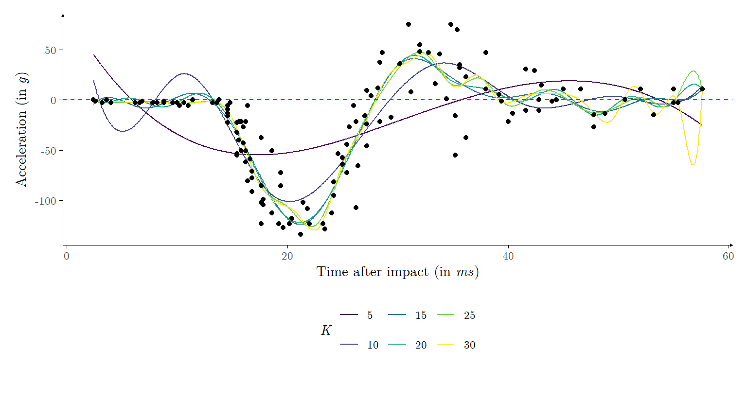
 \] Figure 1 illustrates the estimated mean functions \(\hat{g}(\cdot)\) obtained via maximum likelihood for each \(K\).

Show R code
set.seed(747)
K = c(5, 10, 15, 20, 25, 30)
eval_x = mcycle %>% {seq(from = min(.$times), to = max(.$times), length.out = 1e3 + 1)}
mcycle_fda = 
  lapply(X = seq_along(K),
         FUN = function(x){
           design_basis = create.bspline.basis(rangeval = range(mcycle$times),
                                               norder = 4,
                                               nbasis = K[x])
           design_matrix = design_basis %>%
             getbasismatrix(evalarg = mcycle$times,
                            basisobj = .,
                            nderiv = 0)
           design_matrixf = design_basis %>%
             getbasismatrix(evalarg = eval_x,
                            basisobj = .,
                            nderiv = 0)
           coefficients = design_matrix %>%
             {solve(a = t(.) %*% .,
                    b = t(.) %*% mcycle$accel)}
           return(list(K = K[x],
                       design_matrix = design_matrix,
                       design_matrixf = design_matrixf,
                       coefficients = coefficients,
                       fitted_values = design_matrix %*% coefficients,
                       eval_values = design_matrixf %*% coefficients))
           })
(lapply(X = seq_along(K),
       FUN = function(x){
         data.frame(values = mcycle_fda[[x]]$eval_values,
                    eval_x = eval_x,
                    x = factor(K[x],
                               levels = K))
       }) %>% {do.call(what = rbind,
                       args = .)} %>%
  ggplot(data = .,
         mapping = aes(x = eval_x,
                       y = values,
                       group = x,
                       col = x)) +
  geom_line() +
  theme_classic() +
  theme(text = element_text(size = unit(11, "pt"),
                            family = "LM Roman 10",
                            color = "black"),
        axis.line = element_line(arrow = grid::arrow(length = unit(0.08, "cm"), 
                                                     ends = "last",
                                                     angle = 30,
                                                     type = "closed"),
                                 linewidth = .25),
        axis.ticks = element_line(color = "black",
                                  linewidth = .125),
        legend.position = "bottom") +
  labs(x = substitute(paste("Time after impact (in ", italic("ms"), ")")),
       y = substitute(paste("Acceleration (in ", italic("g"), ")")),
       col = substitute(italic(K))) +
  scale_color_discrete(type = viridis::viridis(n = 6)) +
    geom_hline(col = "red",
               linetype = "dashed",
               yintercept = 0) +
  (mcycle |> geom_point(inherit.aes = F,
                        mapping = aes(x = times,
                                      y = accel)))) / guide_area() + plot_layout(heights = c(4, .5))
Figure 1: Estimated mean functions for the Motorcycle data set, for \(K \in \{5,10,15,20,25,30\}\). The black dots represent the sampled data, and the dashed red line is represents to \(y = 0\).

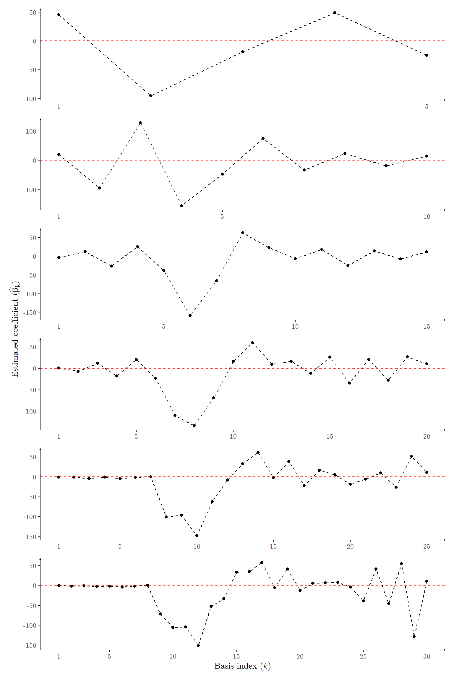
Some remarks can be made with respect to the results of Figure 1: first, we note that for small \(K\) (say \(K \in \{5,10\}\)), the estimated mean function \(\hat{g}(\cdot)\) underfits the data, and is unable to capture localized trends. By contrast, for large \(K\) (say \(K \in \{25,30\}\)), the estimated mean function overfits the data, extrapolating trends which are potentially spurious. This behavior is expected, and is well known in Statistics as the ‘bias-variance tradeoff’. A more interesting remark can be made after we observe Figure 2, which illustrates the estimated coefficient values \(\{\hat{\boldsymbol{\beta}}_\text{ML}\}_k\) for each \(K\).

Show R code
coef_plots =
  lapply(X = seq_along(K),
         FUN = function(x){
           g = mcycle_fda[[x]] %>%
             {data.frame(x = seq_along(.$coefficients),
                         y = .$coefficients) |>
                 ggplot(mapping = aes(x = x,
                                      y = y)) +
                 geom_line(col = "black",
                           linetype = "dashed") +
                 geom_point() +
                 geom_hline(yintercept = 0,
                            linetype = "dashed",
                            col = "red") +
                 scale_x_continuous(breaks = c(1, seq(from = 5, to = K[x], by = 5))) +
                 labs(x = substitute(paste("Basis index (", italic(k), ")")),
                      y = substitute(paste("Estimated coefficient (", hat(beta)[k], ")")))}
           return(list(g = g))
         })
coef_plots[[1]]$g /
coef_plots[[2]]$g /
coef_plots[[3]]$g /
coef_plots[[4]]$g /
coef_plots[[5]]$g /
coef_plots[[6]]$g +
  plot_layout(axes = 'collect',
              guides = 'collect') &
  theme_classic() +
  theme(text = element_text(size = unit(11, "pt"),
                            family = "LM Roman 10",
                            color = "black"),
        axis.line = element_line(arrow = grid::arrow(length = unit(0.08, "cm"), 
                                                     ends = "last",
                                                     angle = 30,
                                                     type = "closed"),
                                 linewidth = .25),
        axis.ticks = element_line(color = "black",
                                  linewidth = .125))
Figure 2: Estimated coefficients for basis expansions of the Motorcycle data set, with \(K \in \{5,10,15,20,25,30\}.\)

It is apparent in Figure 2, particularly for larger \(K\), that some coefficients are very close to zero (though they are not zero). Particularly, this occurs to coefficients corresponding to basis functions which model the start of the mean function (around 15ms after impact), and a few of those which model the latter half of the mean function (around 40ms after impact). This yields mean function estimates close to zero (as can be seen in Figure 1)3. Though the coefficient estimates may be small, and likewise do not possess statistical or practical significance, they are nevertheless not zero (except in essentially pathological cases). As such, our model would include all \(K\) basis functions. A more efficient estimator would automatically identify basis functions whose significance is below a certain threshold and prune those out of the model, yielding a model with only \(K_0 \leq K\) non-zero coefficients, with a comparative performance to the full model. Some procedures for automatic variable selection have been developed, which include the Least Absolute Shrinkage and Selection Operator (LASSO; see Tibshirani (1996)), the Smoothly Clipped Absolute Deviation (SCAD; see Fan and Li (2001)), the Minimax Concave Penalty (MCP; see Zhang (2010)), the Horseshoe prior (see Carvalho, Polson, and Scott (2010)) and Automatic Relevance Determination (ARD; see Tipping (2001)). In Section 2.1 of this vignette we illustrate the application of the ARD procedure to the Motorcyle data set.

The Canadian weather data set

The Canadian weather data set (seen in J. O. Ramsay and Silverman (2002), and available in the fda package in R) consists of measurements obtained across \(N = 35\) Canadian cities: in particular, we focus on the daily average temperatures for each of these cities, averaged from 1960-1994 (hence, for every city we have \(n = 365\) temperature measurements). We denote the day of the measurement as \(t_{ij} \in \{1,2,\ldots,365\}\), and the daily average temperature (in Celsius) as \(y_{ij}\), where the subscript \(i \in \{1,2,\ldots,35\}\) indicates the city to which the measurement corresponds, and the subscript \(j \in \{1,2,\ldots,365\}\) indicates the day to which the measurement corresponds. Therefore, we denote the full data set as \(\{t_{ij},y_{ij}\}^{N,n}_{i = 1,j = 1}\)4. Similarly to the Motorcycle data set context, we denote \(Y_{ij}\) as the random variable corresponding to the average temperature of the \(j\)-th day on the \(i\)-th city, and assume that

\[ \mathbb{E}[Y_{ij}] = g_i(t_{ij}) \quad i \in \{1,\ldots,N\}, j \in \{1,\ldots,n\}. \] A key difference between this formulation and that which is seen in Equation 1 is that the mean function is allowed to vary dependent on the city, that is, we assume that the mean daily temperature profile is different in each city5. Again, we’ll assume that \(Y_{ij} \sim \text{Normal}(g(t_{ij}), 1/\tau_i), \tau_i > 0\), or equivalently

\[ y_{ij} = g_i(t_{ij}) + \tau^{-1/2}_i \varepsilon_{ij} \quad i \in \{1,\ldots,N\}, j \in \{1,\ldots,n\}, \] where \(\varepsilon_{ij} \sim \text{Normal}(0,1), i \in \{1,\ldots,N\}, j \in \{1,\ldots,n\}\). Again we seek to determine estimators \(\hat{g}_i(\cdot)\) for the mean temperature functions, and likewise we assume that the mean temperature functions may be decomposed as linear combinations of a set of basis functions \(\{\phi_k(\cdot)\}_{k = 1}^K\) of the form \[ g_i(t) = \sum^K_{k = 1}\beta_{ik} \phi_k(t), \] for some \(\boldsymbol{\beta}_i \in \mathbb{R}^K\). Unlike the Motorcycle data set application, we consider a different set of basis functions: as we know that the observed functions represent weather observations, we find it ideal that the basis functions accommodate periodic trends that may appear. One ideal family of basis functions in such case is the family of Fourier basis functions (in particular, we adopt \(K = 51\) Fourier basis functions - also including an intercept term - with a periodicity of \(365\), starting at \(t = 1/2\) and ending at \(t = 365 + 1/2\), where the additional \(1/2\) serves to accommodate the transition between the last day of one year and the first day of the next). Disadvantageous to the Fourier approximation, however, is that the Fourier design matrix is not sparse, as the B-spline design matrix may be, and consequently the usage of Fourier basis is more computationally costly. Let \(\boldsymbol{\Phi}_i \in \mathbb{R}^{K \times K}\) and \(\boldsymbol{\phi}_i(t) \in \mathbb{R}^K\) be defined as \[ \boldsymbol{\Phi}_i = \begin{pmatrix} \phi_{1}(t_{i1}) & \phi_{2}(t_{i1}) & \dots & \phi_{K}(t_{i1}) \\ \phi_{1}(t_{i2}) & \phi_{2}(t_{i2}) & \dots & \phi_{K}(t_{i2}) \\ \vdots & \vdots & \ddots & \vdots \\ \phi_{1}(t_{in}) & \phi_{2}(t_{in}) & \dots & \phi_{K}(t_{in}) \end{pmatrix} \quad \text{and} \quad \boldsymbol{\phi}_i(t) = \begin{pmatrix} \phi_1(t) \\ \phi_2(t) \\ \vdots \\ \phi_K(t) \end{pmatrix}. \] Analogously to previous results, we find that the maximum likelihood estimators of the coefficients \(\boldsymbol{\beta}_i\) are \[ \{\hat{\boldsymbol{\beta}}_\text{ML}\}_i = (\boldsymbol{\Phi}_i^\text{T}\boldsymbol{\Phi}_i)^{-1}\boldsymbol{\Phi}^\text{T}_i\mathrm{y}_i \quad i \in \{1,\ldots,N\}, 
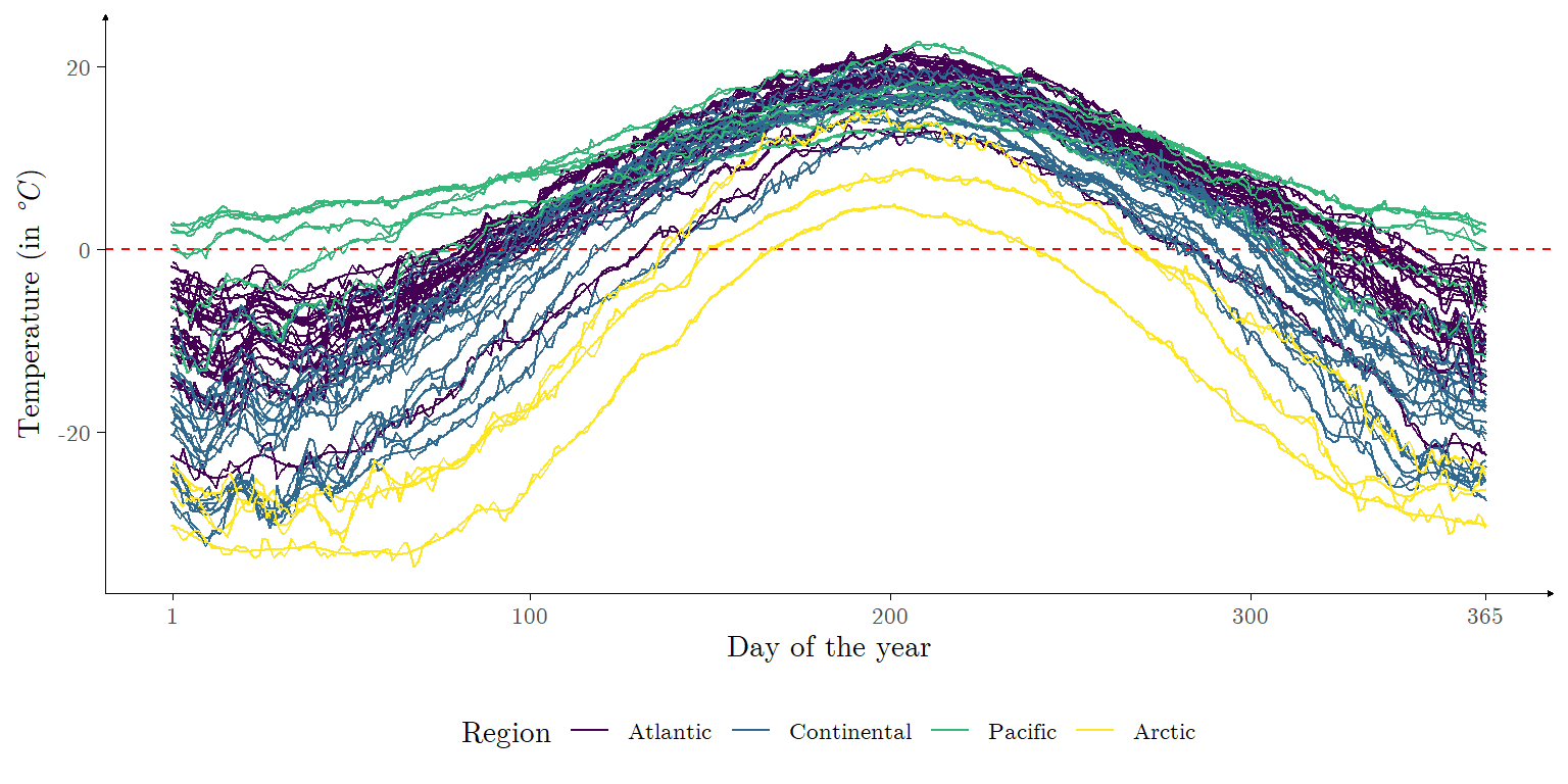
\] assuming \(\boldsymbol{\Phi}_i^\text{T} \boldsymbol{\Phi}_i\) is positive-definite for \(i \in \{1,\ldots,N\}\). The estimated mean functions, as well as the original observed data, are plotted in Figure 3.

Show R code
K_canadian = 51
eval_x_canadian = seq(from = .5, to = 365.5, length.out = 1e3 + 1)
canadianWeather_fda =
  lapply(X = seq_along(CanadianWeather$place),
         FUN = function(x){
           design_basis = create.fourier.basis(rangeval = c(.5, 365.5),
                                               nbasis = K_canadian,
                                               period = 365)
           design_matrix = design_basis %>%
             getbasismatrix(evalarg = 1:365,
                            basisobj = .,
                            nderiv = 0)
           design_matrixf = design_basis %>%
             getbasismatrix(evalarg = eval_x_canadian,
                            basisobj = .,
                            nderiv = 0)
           coefficients = design_matrix %>%
             {solve(a = t(.) %*% .,
                    b = t(.) %*% CanadianWeather$dailyAv[ , x , 1])}
           return(list(K = K_canadian,
                       design_matrix = design_matrix,
                       design_matrixf = design_matrixf,
                       coefficients = coefficients,
                       fitted_values = design_matrix %*% coefficients,
                       eval_values = design_matrixf %*% coefficients,
                       place = CanadianWeather$place[x],
                       day = 1:365))
           })
(lapply(X = seq_along(CanadianWeather$place),
       FUN = function(x){
         data.frame(values = canadianWeather_fda[[x]]$eval_values,
                    eval_x = eval_x_canadian,
                    x = factor(CanadianWeather$place[x],
                               levels = unique(CanadianWeather$place)),
                     region = factor(CanadianWeather$region[x],
                               levels = unique(CanadianWeather$region)),
                     row.names = NULL)
       }) %>% {do.call(what = rbind,
                       args = .)} %>%
  ggplot(data = .,
         mapping = aes(x = eval_x,
                       y = values,
                       group = x,
                       col = region)) +
  geom_line() +
  theme_classic() +
  theme(text = element_text(size = unit(11, "pt"),
                            family = "LM Roman 10",
                            color = "black"),
        axis.line = element_line(arrow = grid::arrow(length = unit(0.08, "cm"), 
                                                     ends = "last",
                                                     angle = 30,
                                                     type = "closed"),
                                 linewidth = .25),
        axis.ticks = element_line(color = "black",
                                  linewidth = .125),
        legend.position = "bottom") +
  labs(x = "Day of the year",
       y = substitute(paste("Temperature (in ", italic("°C"), ")")),
       col = "Region") +
  scale_color_discrete(type = viridis::viridis(n = 4)) +
    scale_x_continuous(breaks = c(1, 100, 200, 300, 365)) +
    geom_hline(yintercept = 0,
                linetype = "dashed",
                col = "red")) +
  (lapply(X = seq_along(CanadianWeather$place),
       FUN = function(x){
         data.frame(values = CanadianWeather$dailyAv[ , x , 1],
                    eval_x = 1:365,
                    x = factor(CanadianWeather$place[x],
                               levels = unique(CanadianWeather$place)),
                     region = factor(CanadianWeather$region[x],
                               levels = unique(CanadianWeather$region)))
       }) %>% {do.call(what = rbind,
                       args = .)} %>%
  geom_line(inherit.aes = F,
            data = .,
            mapping = aes(x = eval_x,
                          y = values,
                          group = x,
                          col = region)))
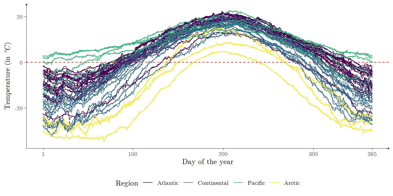
Figure 3: Estimated mean functions for each city in the Canadian weather data set, with \(K = 51\). The original observed data are likewise plotted.

As we deal with a larger number of functions to estimate in this application, we opt to attribute to all expansions the same number of basis functions (\(K = 51\)). As may be seen in Figure 3, the original data set presents a variable region which divides the cities with respect to their corresponding climate zones, although this characteristic is not further explored in this vignette.

Simulated data

In addition to the two data sets presented above, we also consider two distinct scenarios of simulated data. Firstly, we consider a data set comprised of \(N\) functions sampled \(n\) times each, generated from a cubic B-spline basis set of functions, with equidistant knots starting at \(0\) and ending at \(1\), such that we have 10 basis functions, however only 6 have non-zero true coefficients. The sampling design is regular (see the footnotes) in the interval \([0,1]\). Our goal with this simulation is to determine the accuracy of the estimated coefficients for the ARD procedure. The data is generated as follows

\[ y_{ij} = \boldsymbol{\phi}^\text{T}(t_{ij})\begin{pmatrix} -2 \\ 0 \\ 3/2 \\ 3/2 \\ 0 \\ -1 \\ -1/2 \\ -1 \\ 0 \\ 0 \end{pmatrix} + \tau^{-1/2}\varepsilon_{ij}, \tag{5}\] where \(\boldsymbol{\phi}(t)\) is as in Equation 4 and \(\tau = 25\). Figure 4 illustrates one generated replication of this data set.

Show R code
set.seed(23121998)
replication_1 = 1000
N_1 = 10
n_1 = 10
t_1 = seq(from = 0, to = 1, length.out = n_1)
tau_1 = .2 ** -2
beta_1 = c(-2, 0, 3/2, 3/2, 0, -1, -1/2, -1, 0, 0)
K_1 = length(beta_1)
beta_in_1 = which(beta_1 != 0)
beta_out_1 = which(beta_1 == 0)
Phi_1 = create.bspline.basis(rangeval = c(0, 1),
                             norder = 4,
                             nbasis = K_1) %>%
  getbasismatrix(evalarg = t_1,
                 basisobj = .,
                 nderiv = 0)
mean_1 = Phi_1 %*% beta_1
sim_data_1 = lapply(X = 1:N_1,
                    FUN = function(x){
                      y = mean_1 + (tau_1 ** (-1/2)) * rnorm(n = n_1)
                      return(y)
                    })
(lapply(X = 1:N_1,
        FUN = function(x){
          data.frame(x = t_1,
                     y = sim_data_1[[x]],
                     ind = factor(x, levels = 1:N_1))
        })) %>% do.call(what = rbind,
                        args = .) |>
  ggplot(mapping = aes(x = x,
                       y = y,
                       group = ind,
                       col = ind)) +
  geom_line() +
  theme_classic() +
  theme(text = element_text(size = unit(11, "pt"),
                            family = "LM Roman 10",
                            color = "black"),
        axis.line = element_line(arrow = grid::arrow(length = unit(0.08, "cm"), 
                                                     ends = "last",
                                                     angle = 30,
                                                     type = "closed"),
                                 linewidth = .25),
        axis.ticks = element_line(color = "black",
                                  linewidth = .125),
        legend.position = "none") +
  labs(x = substitute(paste(italic(t)[ij])),
       y = substitute(paste(italic(y)[ij]))) +
  scale_color_discrete(type = viridis::viridis(n = N_1)) +
    scale_x_continuous(breaks = c(0, .5, 1),
                       labels = c("0", "1/2", "1")) +
    geom_hline(yintercept = 0,
                linetype = "dashed",
                col = "red")
Figure 4: \(N = 10\) functions sampled at \(n = 10\) instants according to Equation 5

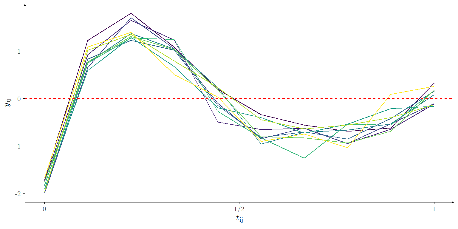
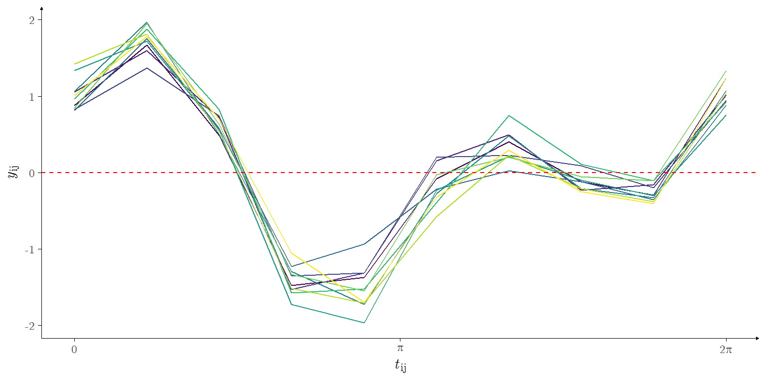
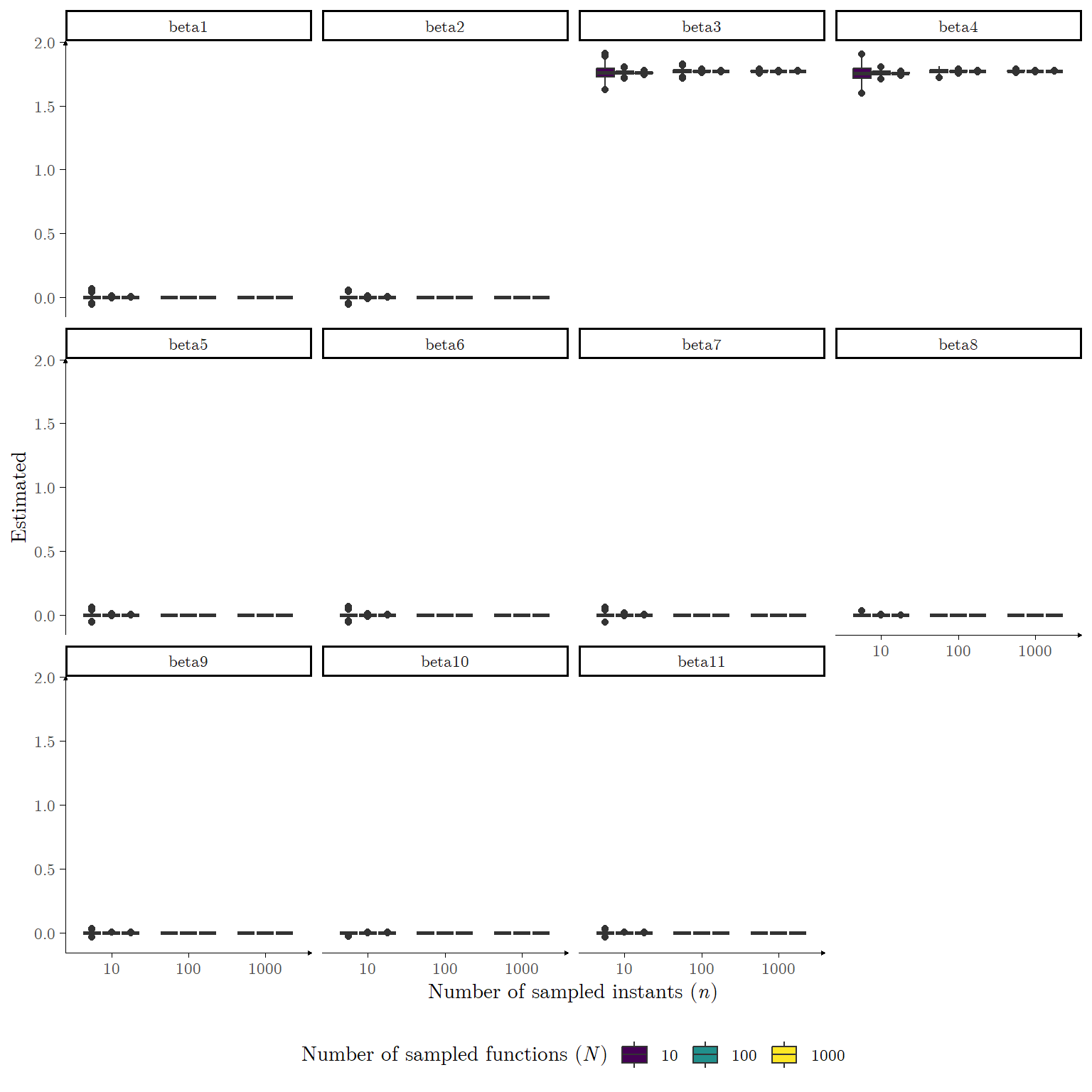
For the second simulation, we generated a data set composed of \(N\) functions sampled \(n\) times each (again, the sampling design is regular in the interval \([0,2\pi]\)), where the mean curve is the sum of two trigonometric functions, as in

\[ y_{ij} = \cos(t_{ij}) + \sin(2 t_{ij}) + \tau^{-1/2}\varepsilon_{ij}, \tag{6}\]

with \(\tau = 25\). Unlike the previous simulation, we consider the mean function expansions \(\hat{g}_i(\cdot)\) as resulting from a linear combination of \(K = 10\) Fourier basis functions, with periodicity equal to \(2\pi\), starting at \(0\). Similarly to the previous simulation, this implies that the coefficients in the resulting expansion must be non-zero for only two of the basis functions. Figure 5 illustrates one generated replication of this data set.

Show R code
set.seed(12231998)
replication_2 = 1000
N_2 = 10
n_2 = 10
t_2 = seq(from = 0, to = 2 * pi, length.out = n_2)
tau_2 = .2 ** -2
beta_2 = c(0, 0, 1, 1, 0, 0, 0, 0, 0, 0, 0)
K_2 = length(beta_2)
beta_in_2 = which(beta_2 != 0)
beta_out_2 = which(beta_2 == 0)
mean_2 = cos(t_2) + sin(2 * t_2)
sim_data_2 = lapply(X = 1:N_2,
                    FUN = function(x){
                      y = mean_2 + (tau_2 ** (-1/2)) * rnorm(n = n_2)
                      return(y)
                    })
(lapply(X = 1:N_2,
        FUN = function(x){
          data.frame(x = t_2,
                     y = sim_data_2[[x]],
                     ind = factor(x, levels = 1:N_2))
        })) %>% do.call(what = rbind,
                        args = .) |>
  ggplot(mapping = aes(x = x,
                       y = y,
                       group = ind,
                       col = ind)) +
  geom_line() +
  theme_classic() +
  theme(text = element_text(size = unit(11, "pt"),
                            family = "LM Roman 10",
                            color = "black"),
        axis.line = element_line(arrow = grid::arrow(length = unit(0.08, "cm"), 
                                                     ends = "last",
                                                     angle = 30,
                                                     type = "closed"),
                                 linewidth = .25),
        axis.ticks = element_line(color = "black",
                                  linewidth = .125),
        legend.position = "none") +
  labs(x = substitute(paste(italic(t)[ij])),
       y = substitute(paste(italic(y)[ij]))) +
  scale_color_discrete(type = viridis::viridis(n = N_1)) +
    scale_x_continuous(breaks = c(0, pi, 2 * pi),
                       labels = expression("0", pi, paste("2", pi))) +
    geom_hline(yintercept = 0,
                linetype = "dashed",
                col = "red")
Figure 5: \(N = 10\) functions sampled at \(n = 10\) instants according to Equation 6

For both simulations we’ll consider 9 possible scenarios, with varying values for \(N\) and \(n\), whice are presented in Table 1.

Scenario N n
1 10 10
2 10 100
3 10 1000
4 100 10
5 100 100
6 100 1000
7 1000 10
8 1000 100
9 1000 1000
Table 1: Scenarios for the simulation studies.

Setup

This vignette is primarily concerned with presenting an approach to sparse representation of Functional Data utilizing the Automatic Relevance Determination (ARD) framework, itself only a topic in the wider Sparse Bayesian Learning (SBL) context. More precisely, our aim herein is to replicate some of the studies in Sousa, Souza, and Dias (2024) and Cruz, Souza, and Sousa (2024) (the former moreso than the latter, as we do not account for any correlation structure in the functions). The goal of these previous studies was to provide an adaptive Bayesian procedure to select the bases for functional data representation, the latter also extending the results of the former by including a correlation structure for the functional data, and delineating an estimation procedure utilizing the Variational Bayes (VB) approach. It did so by including a collection of Bernoulli random variables (denoted \(Z_{k}\)), each associated with one particular term in the basis expansion in Equation 3, resulting in the form \(\tilde{\beta}_{k} = Z_{k} \beta_{k}\), such that \(\mathbb{P}(\tilde{\beta}_{k} = 0) > 0\). The ARD approach, which is presented subsequently, similarly works as Bayesian model.

Automatic Relevance Determination

The ARD approach attributes the following hierarchical Bayesian model:

\[ \begin{aligned} y(t_{j}) \vert \{\beta_{k}\}, \tau & \sim \text{Normal}\Bigg(\sum^K_{k = 1}\beta_{k}\phi_k(t_{j}), \tau^{-1}\Bigg) & j \in \{1,\ldots,n\} \\ {\beta}_{k} \vert \alpha_{k} & \sim \text{Normal}(0,\alpha_{k}^{-1}) & k \in \{1,\ldots,K\}. \end{aligned} \] Where \(\{\alpha_{k}\}\) (greater than zero) are hyperparameters which dictate the concentration of the coefficients around zero, whilst \(\tau\) (also greater than zero) is a hyperparameter which dictates the precision of the sampled observations. In adopting the empirical Bayes approach to estimate the model, we aim to determine the hyperparameter values which maximize the distribution of the observations points marginalized over the coefficients \(\{\beta_{k}\}\). Tipping (2001) proposes a straightforward set of update equations for the hyperparameters (as well as for the coefficients, which are estimated via their maximum a posteriori value). These are as follows:

\[ \hat{\boldsymbol{\beta}} = \hat{\tau} \boldsymbol{\Sigma}\Phi^\text{T}\mathrm{y} \tag{7}\]

\[ \hat{\alpha}_k = \frac{\gamma_k}{\hat{\beta}_k^2} \tag{8}\]

\[ \frac{1}{\hat{\tau}} = \frac{\lvert\lvert \textbf{y} - \Phi \hat{\boldsymbol{\beta}}\rvert\rvert^2}{n - \sum^K_{k = 1}\gamma_{k}} \quad k \in \{1,\ldots,K\} \tag{9}\]

where

\[ \boldsymbol{\Sigma} = (\text{diag}(\hat{\alpha}) + \hat{\tau} \boldsymbol{\Phi}^\text{T}\boldsymbol{\Phi})^{-1} \tag{10}\]

\[ \gamma_{k} = 1 - \hat{\alpha}_{k}\Sigma_{kk} \quad k \in \{1,\ldots,K\}. \tag{11}\]

Tipping (2001) likewise demonstrates that, under certain circumstances, \(\hat{\alpha}_k \approx \infty\), under which condition the prior distribution of \(\beta_k \vert \alpha_k\) is approximately degenerate at 0 (as is the consequent posterior). We provide an algorithm for the estimation of an ARD model, given the above updating equations:

Initialization. Enter a valid response vector \(\mathrm{y}\) and a valid predictor matrix \(\boldsymbol{\Phi}\). Set a cutoff value \(M > 0\) such that, if \(\hat{\alpha}_k > M\), \(\hat{\beta}_k = 0\). Set initial values for the estimators \(\hat{\tau} = \tau_0\) and \(\hat{\alpha} = \alpha_0\). Thereafter, perform the following steps in sequence.

  1. Compute the quantities in Equation 10 and Equation 11.
  2. Update \(\hat{\beta}_k\) (for variables still in the model) according to Equation 7.
  3. Update \(\hat{\alpha}_k\) (for variables still in the model) and \(\hat{\tau}\) according to Equation 8 and Equation 9.
  4. For every \(k \in \{1,\ldots,K\}\) if \(\hat{\alpha}_{k} > M\), remove the \(k\)-th variable from the model.
  5. Check the convergence of the estimates. If convergence has occurred, stop. Else, return to step (1).

The function ard_model() in the chunk below performs the estimating procedure.

Show R code
ard_model = function(y,
                     Phi,
                     tau_ini = 1,                             
                     alpha_ini = rep(x = 1,
                                     times = ncol(Phi)),
                     max_iter = 1e3,
                     tol = 1e-8,
                     cutoff = 1e4)
{
  time = Sys.time()
  n = length(y)
  K = ncol(Phi)
  
  tau = tau_ini
  alpha = alpha_ini
  keep = !logical(K)
  
  beta_est = rep(0, times = K)
  gamma_est = rep(0, times = K)
  
  iter = 1
  cond = Inf
  beta_est0 = beta_est + Inf
  
  while((iter < max_iter) & (abs(cond) > tol))
  {
    Phi_keep = Phi[,keep]
    
    A = diag(alpha[keep])
    
    Sigma = solve(A + tau * t(Phi_keep) %*% Phi_keep)
    
    beta_est[keep] = tau * Sigma %*% t(Phi_keep) %*% y
    
    gamma_est[keep] = 1 - alpha[keep] * diag(Sigma)
    
    alpha[keep] = gamma_est[keep] / (beta_est[keep] ** 2)
    tau = (n - sum(gamma_est[keep])) / sum((y - Phi_keep %*% beta_est[keep]) ** 2)
    
    keep = ifelse(test = alpha < cutoff, yes = T, no = F)
    
    beta_est[!keep] = 0
    alpha[!keep] = Inf
    
    iter %<>% + 1
    
    cond = sum((beta_est - beta_est0) ** 2) 
    beta_est0 = beta_est
  }
  
  fitted_values = Phi[,keep] %*% beta_est[keep]
  R2_adj0 = 1 - ((n - 1) / (n - length(gamma_est[keep]))) * (sum((y - fitted_values) ** 2) / sum((y - mean(y)) ** 2))
  R2_adj = 1 - ((n - 1) / (n - sum(gamma_est[keep]))) * (sum((y - fitted_values) ** 2) / sum((y - mean(y)) ** 2))
  
  time %<>% {Sys.time() - .}
  
  return(list(iter = iter,
              tau = tau,
              alpha = alpha[keep],
              beta = beta_est[keep],
              gamma = gamma_est[keep],
              keep = which(keep),
              time = time,
              fitted_values = fitted_values,
              R2_adj = R2_adj,
              R2_adj0 = R2_adj0))
}

Bishop (2006) suggests utilizing \(\{\gamma_k\}\), defined in Equation 11, as a measure of the model complexity, defining the effective degrees of freedom of the model as \[ \text{df}_\text{eff} = \sum^K_{k = 1}\gamma_k. \] Note that, if the \(k\)-th coefficient is included in the model, \(\gamma_k \in [0,1]\), whereas if its not included, \(\gamma_k = 0\). In the following section we’ll utilize two distinct measures of quality of fit for our models. First, we define the usual adjusted \(R\) squared as \[ R^2_\text{adj} = 1 - \frac{n - 1}{n - \hat{K}_0} \frac{\sum^n_{i = 1}(y_i - \hat{g}(t_i))^2}{\sum^n_{i = 1}(y_i - \bar{y}^2)}, \] where \[ \hat{K}_0 = K - \sum^K_{k = 1} \textbf{1}_{\{0\}}(\hat{\beta}_k), \] that is, \(\hat{K}_0 \in [0,K]\) is the number of non-zero coefficients in the estimated model. We additionally define \[ \widetilde{R}^2_\text{adj} = 1 - \frac{n - 1}{n - \text{df}_\text{eff}} \frac{\sum^n_{i = 1}(y_i - \hat{g}(t_i))^2}{\sum^n_{i = 1}(y_i - \bar{y}^2)}. \] Note that \(\text{df}_\text{eff} \in [0,K_0]\), hence \(\widetilde{R}^2_\text{adj} \geq R^2_\text{adj}\).

Applications and Simulations

Application I

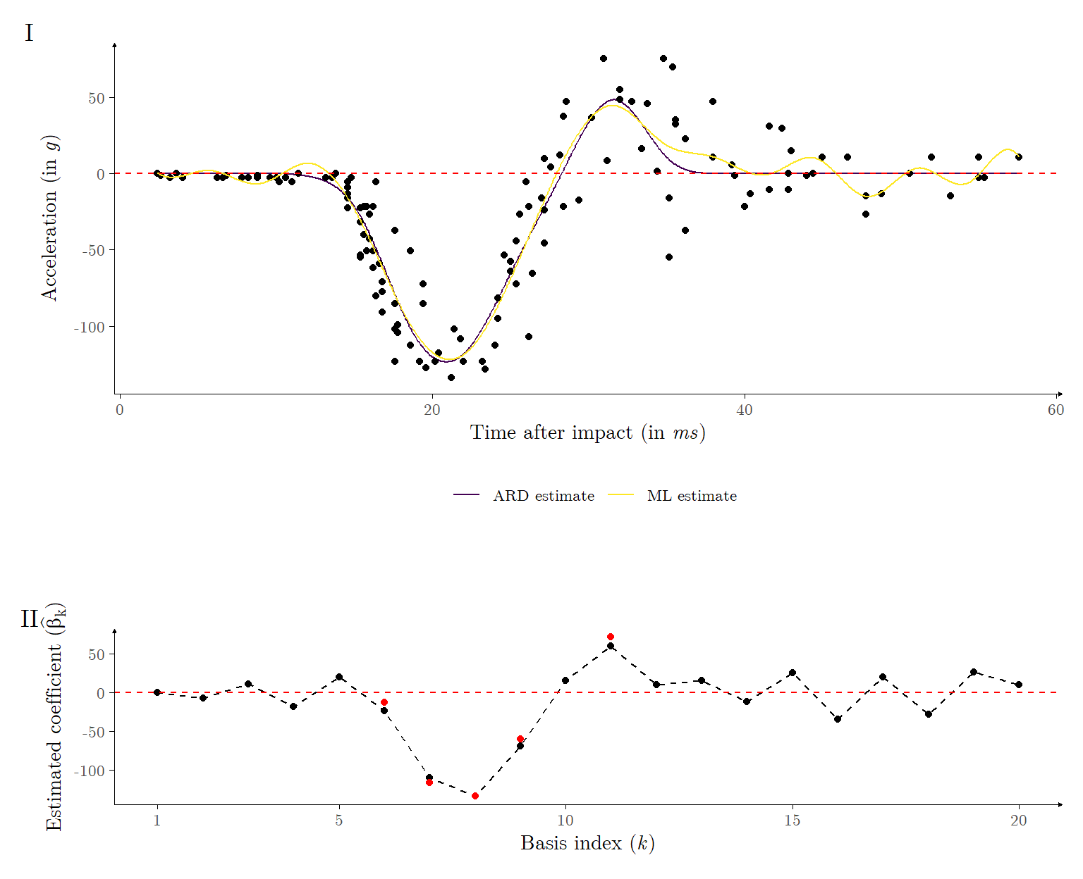
For the Motorcycle data set application, we utilize the cubic B-spline expansion composed of \(K = 20\) basis functions. We first set the cutoff \(M\) in the ARD algorithm to an arbitrarily large value (\(\log_{10}M = 4\)), in which case the the estimated model had \(\hat{K}_0 = 7\) non-zero coefficients. However, by setting the cutoff to a lower value (\(\log_{10} M = -2\)) we found the model’s adjusted \(R\) squared had improved, with the model having only \(\hat{K}_0 = 5\) non-zero coefficients. It may therefore be of interest to view the cutoff value \(M\) as a tuning parameter. Figure 6 illustrates the estimated model.

Show R code
ind = 4
mcycle_ard = ard_model(y = mcycle$accel,
                       Phi = mcycle_fda[[ind]]$design_matrix,
                       cutoff = 1e-2)
(mcycle_ard %>% {data.frame(eval_x = eval_x,
                           eval_values = mcycle_fda[[ind]]$design_matrixf[,.$keep] %*% .$beta)} |>
  ggplot(mapping = aes(x = eval_x,
                       y = eval_values,
                       col = "ARD estimate")) +
  geom_line() +
  (mcycle |> geom_point(inherit.aes = F,
                        mapping = aes(x = times,
                                      y = accel))) +
  (mcycle_fda[[ind]] %>% {data.frame(eval_x = eval_x,
                                   eval_values = .$design_matrixf %*% .$coefficients)} |>
     geom_line(inherit.aes = F,
               mapping = aes(x = eval_x,
                             y = eval_values,
                             col = "ML estimate"))) +
  theme_classic() +
  theme(text = element_text(size = unit(11, "pt"),
                            family = "LM Roman 10",
                            color = "black"),
        axis.line = element_line(arrow = grid::arrow(length = unit(0.08, "cm"), 
                                                     ends = "last",
                                                     angle = 30,
                                                     type = "closed"),
                                 linewidth = .25),
        axis.ticks = element_line(color = "black",
                                  linewidth = .125),
        legend.position = "bottom") +
  labs(x = substitute(paste("Time after impact (in ", italic("ms"), ")")),
       y = substitute(paste("Acceleration (in ", italic("g"), ")")),
       col = "") +
    geom_hline(col = "red",
               linetype = "dashed",
               yintercept = 0) +
    scale_color_discrete(type = viridis::viridis(2))) /
  (guide_area()) / 
(coef_plots[[ind]]$g +
  theme_classic() +
  theme(text = element_text(size = unit(11, "pt"),
                            family = "LM Roman 10",
                            color = "black"),
        axis.line = element_line(arrow = grid::arrow(length = unit(0.08, "cm"), 
                                                     ends = "last",
                                                     angle = 30,
                                                     type = "closed"),
                                 linewidth = .25),
        axis.ticks = element_line(color = "black",
                                  linewidth = .125)) +
  (mcycle_ard %>% {data.frame(x = .$keep,
                              y = .$beta) |>
      geom_point(inherit.aes = F,
                 mapping = aes(x = x,
                               y = y),
                 col = "red")})) + plot_layout(heights = c(4, .5, 2)) +
  plot_annotation(tag_levels = 'I')
Figure 6: Panel I: Estimated mean functions for the Motorcycle data set, with \(K = 20\), obtained via the ARD procedure and Maximum Likelihood (ML). Panel II: Estimated coefficients for basis expansions of the Motorcycle data set, with \(K = 20\). The black points are those obtained via ML, whilst the red points are those obtained via ARD. Estimates equal to zero are ommited.

The observed adjusted \(R\) squared values were \(R^2_\text{adj} \approx 0.7858\) and \(\widetilde{R}^2_\text{adj} \approx 0.7864\). Note that the ARD procedure selects basis functions which model the interval where the acceleration showcases a valley followed by a peak, effectively capturing the most apparent trends in the data whilst utilizing only 25% of the originally proposed basis functions. The basis functions which correspond to the beginning of the mean function (around 15\(ms\) after impact), where the data is approximately inert, are removed, as are those which model the tail end of the mean function (around 40\(ms\) after impact), as was expected. These results follow closely those obtained in Cruz, Souza, and Sousa (2024).

Application II

For the Canadian weather application, as previously stated, we utilized \(K = 51\) Fourier basis functions, starting at \(1/2\) and ending at \(365 + 1/2\), with periodicity of \(365\). We adopted as the cutoff parameter the value of \(\log_{10} M = 4\), though we also found that lower values (e.g. \(\log_{10} M = 2\)) exhibit similar overall performance. Figure 7 illustrates the estimated mean functions.

Show R code
canadianWeather_ard = lapply(X = seq_along(CanadianWeather$place),
                             FUN = function(x){
                               ard_model(y = CanadianWeather$dailyAv[ , x, 1],
                                         Phi = canadianWeather_fda[[x]]$design_matrix,
                                         cutoff = 1e4)
                             })
(canadianWeather_ard %>% {lapply(X = seq_along(CanadianWeather$place),
        FUN = function(x){
          data.frame(eval_x = eval_x_canadian,
                     values = canadianWeather_fda[[x]]$design_matrixf[,.[[x]]$keep] %*% .[[x]]$beta,
                     x = factor(CanadianWeather$place[x],
                               levels = unique(CanadianWeather$place)),
                     region = factor(CanadianWeather$region[x],
                               levels = unique(CanadianWeather$region)),
                     row.names = NULL)
        })} %>% {do.call(what = rbind,
                       args = .)} %>%
  ggplot(data = .,
         mapping = aes(x = eval_x,
                       y = values,
                       group = x,
                       col = region)) +
    geom_line() +
    theme_classic() +
  theme(text = element_text(size = unit(11, "pt"),
                            family = "LM Roman 10",
                            color = "black"),
        axis.line = element_line(arrow = grid::arrow(length = unit(0.08, "cm"), 
                                                     ends = "last",
                                                     angle = 30,
                                                     type = "closed"),
                                 linewidth = .25),
        axis.ticks = element_line(color = "black",
                                  linewidth = .125),
        legend.position = "bottom") +
  labs(x = "Day of the year",
       y = substitute(paste("Temperature (in ", italic("°C"), ")")),
       col = "Region") +
  scale_color_discrete(type = viridis::viridis(n = 4)) +
    scale_x_continuous(breaks = c(1, 100, 200, 300, 365)) +
    geom_hline(yintercept = 0,
                linetype = "dashed",
                col = "red")) +
  (lapply(X = seq_along(CanadianWeather$place),
       FUN = function(x){
         data.frame(values = CanadianWeather$dailyAv[ , x , 1],
                    eval_x = 1:365,
                    x = factor(CanadianWeather$place[x],
                               levels = unique(CanadianWeather$place)),
                     region = factor(CanadianWeather$region[x],
                               levels = unique(CanadianWeather$region)),
                     row.names = NULL)
       }) %>% {do.call(what = rbind,
                       args = .)} %>%
  geom_line(inherit.aes = F,
            data = .,
            mapping = aes(x = eval_x,
                          y = values,
                          group = x,
                          col = region)))
time_canadian_ARD = canadianWeather_ard %>% {lapply(X = seq_along(CanadianWeather$place), FUN = function(x){.[[x]]$time})} |> unlist() |> sum()
p_basis_canadian_ARD = 100 * (canadianWeather_ard %>% {lapply(X = seq_along(CanadianWeather$place), FUN = function(x){length(.[[x]]$keep)})} |> unlist() |> mean()) / K_canadian
R2_adj_basis_canadian_ARD = canadianWeather_ard %>% {lapply(X = seq_along(CanadianWeather$place), FUN = function(x){.[[x]]$R2_adj})} |> unlist() |> mean()
R2_adj0_basis_canadian_ARD = canadianWeather_ard %>% {lapply(X = seq_along(CanadianWeather$place), FUN = function(x){.[[x]]$R2_adj0})} |> unlist() |> mean()
Figure 7: Estimated mean functions for each city in the Canadian weather data set, with \(K = 51\), obtained via the ARD procedure. The original observed data are likewise plotted.

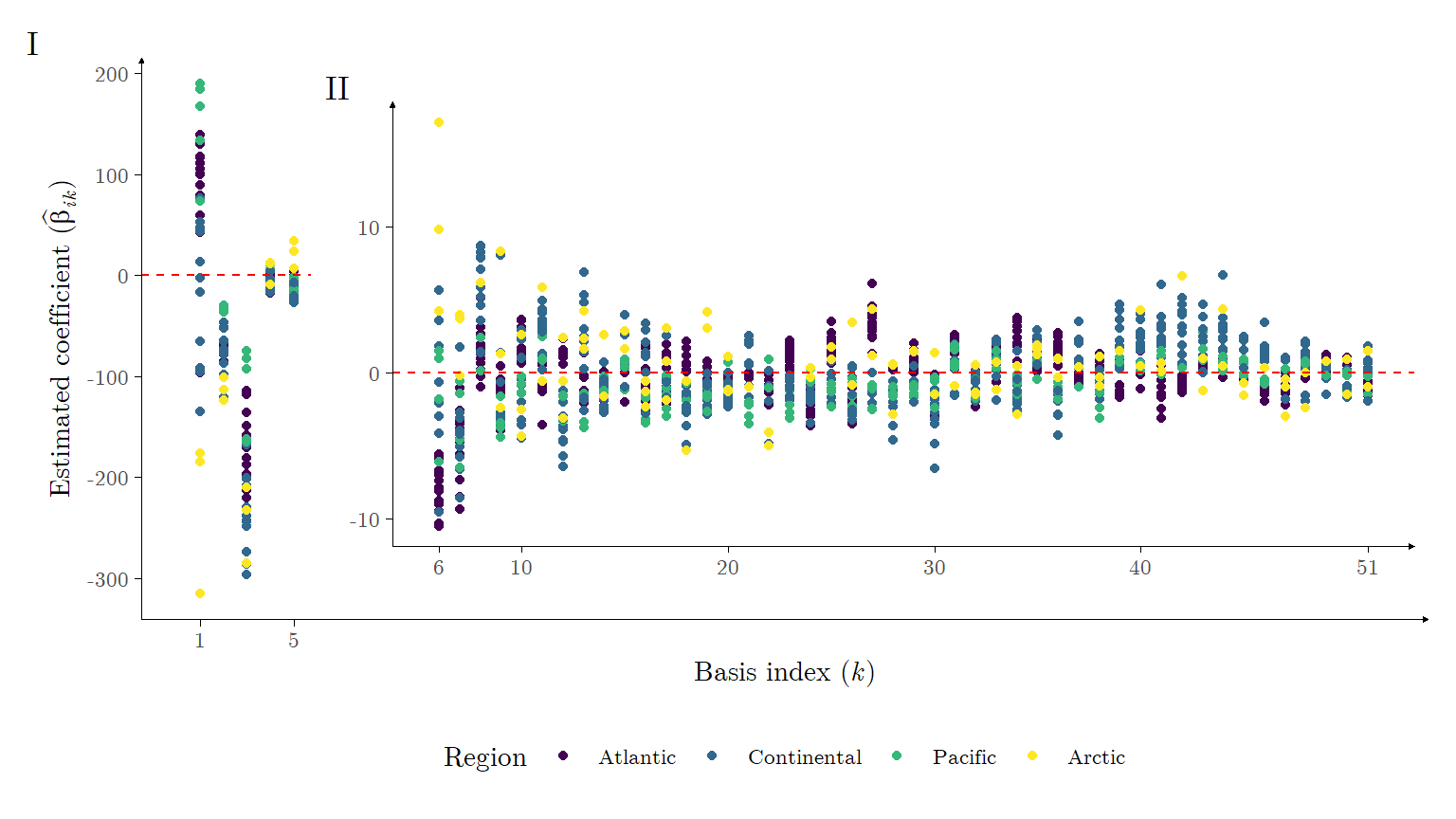
We note that the ARD estimation procedure for all functions took approximately 4.8932 seconds to finish, and kept on average approximately \(74.8459\%\) of the original basis functions per estimated mean function, resulting in an average adjusted \(R\) squared of \(R^2_\text{adj} \approx 0.9968\) and \(\widetilde{R}^2_\text{adj} \approx 0.9969\). Figure 8 exhibits the coefficients corresponding to the estimated mean functions.

Show R code
p_canadian_1 = (lapply(X = seq_along(CanadianWeather$place),
       FUN = function(x){
         canadianWeather_ard[[x]] %>%
         {data.frame(kept = .$keep,
                    region = factor(CanadianWeather$region[x],
                                    levels = unique(CanadianWeather$region)),
                    beta = .$beta,
                    row.names = NULL)}
       }) %>% do.call(what = rbind,
                      args = .) |>
  ggplot(mapping = aes(x = kept,
                       y = beta,
                       col = region)) +
  geom_point() +
  theme_classic() +
  theme(text = element_text(size = unit(11, "pt"),
                            family = "LM Roman 10",
                            color = "black"),
        axis.line = element_line(arrow = grid::arrow(length = unit(0.08, "cm"), 
                                                     ends = "last",
                                                     angle = 30,
                                                     type = "closed"),
                                 linewidth = .25),
        axis.ticks = element_line(color = "black",
                                  linewidth = .125),
        legend.position = "bottom") +
  labs(x = substitute(paste("Basis index (", italic(k), ")")),
       y = substitute(paste("Estimated coefficient (", hat(beta)[italic(ik)], ")")),
       col = "Region") +
  scale_color_discrete(type = viridis::viridis(4)) +
    scale_x_continuous(breaks = c(1, 5)) +
    geom_hline(col = "red", linetype = "dashed", yintercept = 0))
p_canadian_2 = (lapply(X = seq_along(CanadianWeather$place),
       FUN = function(x){
         canadianWeather_ard[[x]] %>%
         {data.frame(kept = .$keep,
                    region = factor(CanadianWeather$region[x],
                                    levels = unique(CanadianWeather$region)),
                    beta = .$beta,
                    row.names = NULL)}
       }) %>% do.call(what = rbind,
                      args = .) |>
     subset(kept > 5) |>
  ggplot(mapping = aes(x = kept,
                       y = beta,
                       col = region)) +
  geom_point() +
  theme_classic() +
  theme(text = element_text(size = unit(11, "pt"),
                            family = "LM Roman 10",
                            color = "black"),
        axis.line = element_line(arrow = grid::arrow(length = unit(0.08, "cm"), 
                                                     ends = "last",
                                                     angle = 30,
                                                     type = "closed"),
                                 linewidth = .25),
        axis.ticks = element_line(color = "black",
                                  linewidth = .125),
        legend.position = "none",
        axis.title.y = element_blank(),
        axis.title.x = element_blank()) +
  labs(x = substitute(paste("Basis index (", italic(k), ")")),
       y = substitute(paste("Estimated coefficient (", hat(beta)[italic(ik)], ")")),
       col = "Region") +
  scale_color_discrete(type = viridis::viridis(4)) +
    scale_x_continuous(breaks = c(6, 10, 20, 30, 40, 51)) +
    geom_hline(col = "red", linetype = "dashed", yintercept = 0))
p_canadian_1 + inset_element(p_canadian_2, .132, .05, 1, 1) +
  plot_annotation(tag_levels = 'I')
Figure 8: Panel I: Estimated coefficients for basis expansions of the Canadian weather data set, with \(K = 51\), obtained via the ARD procedure. Panel II: Inset zoom-in of the former Panel for basis indexes between 6 and 51.

As is expected when utilizing a Fourier basis expansion, the coefficients associated with basis’ with higher frequencies are smaller in absolute value, some close to zero. Nevertheless, we found that these basis’ are only removed from the model when the cutoff is lower than \(\log_{10} M = 0\). Moreover, the model obtained with \(\log_{10} M = 0\) has worsened average adjusted \(R\) squared. Consequently, we opted to stick with the cutoff of \(\log_{10} M = 4\). Table 2 presents some diagnostic values obtained from the model (\(R^2_\text{adj}\) is denoted as R2 I and \(\widetilde{R}^2_\text{adj}\) is denoted as R2 II), discriminated by city. Once more, the results followed closely those obtained in Cruz, Souza, and Sousa (2024).

Table 2: Some diagnostic values obtained by the application of the ARD procedure, discriminated by city.
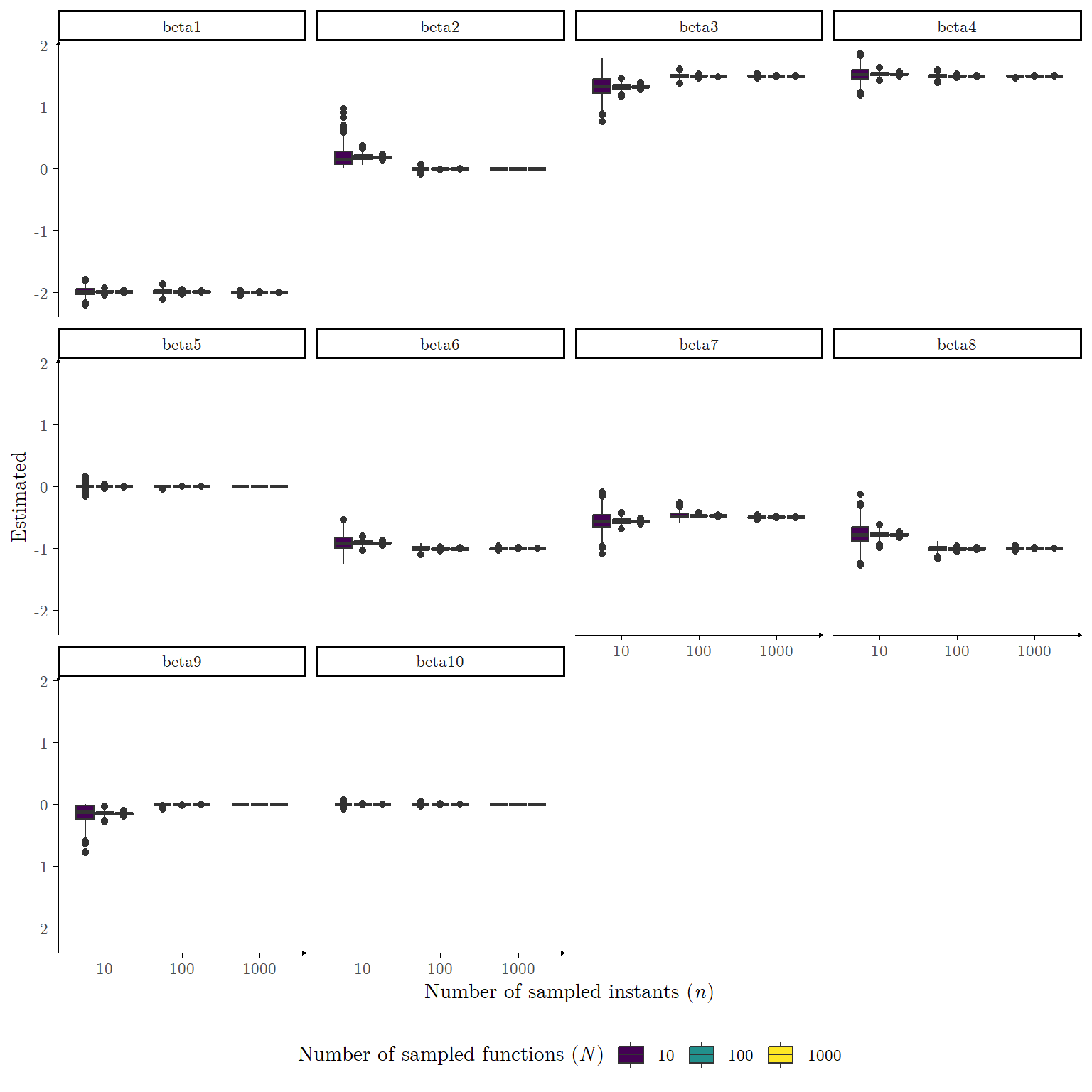
Simulation Study I

For each simulation study scenario, we replicated \(\textbf{R} = 1000\) data sets, obtaining a model for each via Automatic Relevance Determination. Let \(K\) denote the number of basis functions, \(K_0\) denote the number of non-zero coefficients, \(\hat{\beta}_{ijr}(N,n)\) denote the estimated coefficient corresponding to the \(j\)-th basis function of the \(i\)-th functional observation obtained on the \(r\)-th replication of the scenario with number of functional observations \(N\) and number of sampled instants \(n\) (analogously for \(\hat{\tau}_{ir}(N,n)\)) we consider of interest the following measures: \[ \hat{\beta}_{jr}(N,n) = \frac{1}{N}\sum^N_{i = 1}\hat{\beta}_{ijr}(N,n) \tag{12}\] \[ \hat{\tau}_r(N,n) = \frac{1}{N}\sum^N_{i = 1}\hat{\tau}_{ir}(N,n) \tag{13}\] \[ \widehat{\text{SEN}}_r(N,n) = \frac{1}{N (K - K_0)}\Bigg(\sum_{\{(i,j) : \beta_{ij}(n) \neq 0\}}\textbf{1}_{\{0\}^C}(\hat{\beta}_{ijr}(N,n))\Bigg) \tag{14}\]

\[ \widehat{\text{SPE}}_r(N,n) = \frac{1}{NK_0}\sum_{\{(i,j) : \beta_{ij} = 0\}}\textbf{1}_{\{0\}}(\hat{\beta}_{ijr}(N,n)) \tag{15}\] \[ \widehat{\text{ACC}}_r(N,n) = \frac{1}{NK}\Bigg(\sum_{\{(i,j) : \beta_{ij} = 0\}}\textbf{1}_{\{0\}}(\hat{\beta}_{ijr}(N,n)) + \sum_{\{(i,j) : \beta_{ij} \neq 0\}}\textbf{1}_{\{0\}^c}(\hat{\beta}_{ijr}(N,n))\Bigg). \tag{16}\]

Equation 12 and Equation 13 measure the average values obtained for the \(j\)-th coefficient in the basis expansion and the average precision parameter, respectively, for the \(r\)-th replication. Equation 14 measures the sensibility (percentage of non-zero coefficients which were estimated as non-zero) of the \(r\)-th replication. Equation 15 measures the specificity (percentage of zero coefficients which were estimated as zero) of the \(r\)-th -replication. Lastly, Equation 16 measures the overall accuracy of the \(r\)-th -replication. The R chunk provided below performs \(\textbf{R} = 1000\) replications of the nine scenarios for the first Simulation framework. For this simulation we adopted as the cutoff in the ARD procedure the value of \(\log_{10} M = 1\).

Show R code
set.seed(23121998)
N_sim_1 = rep(c(10, 100, 1000), each = 3)
n_sim_1 = rep(c(10, 100, 1000), times = 3)
df_sim_1 = 
  lapply(X = seq_along(N_sim_1),
         function(q){
          N_1 = N_sim_1[q]
          n_1 = n_sim_1[q]
          t_1 = seq(from = 0, to = 1, length.out = n_1)
          Phi_1 = create.bspline.basis(rangeval = c(0, 1),
                                       norder = 4,
                                       nbasis = K_1) %>%
            getbasismatrix(evalarg = t_1,
                           basisobj = .,
                           nderiv = 0)
          mean_1 = Phi_1 %*% beta_1
          sim_data_total_1 = lapply(X = 1:replication_1, FUN = function(z){
          sim_data_1 = lapply(X = 1:N_1,
                            FUN = function(x){
                              beta_est = numeric(length = K_1)
                              y = mean_1 + (tau_1 ** (-1/2)) * rnorm(n = n_1)
                              est = ard_model(y = y,
                                              Phi = Phi_1,
                                              cutoff = 1e1)
                              beta_est[est$keep] = est$beta
                              sen = sum(est$keep %in% beta_in_1)
                              spe = sum((1:K_1)[-c(est$keep)] %in% beta_out_1)
                              acc = sen + spe
                              tau_est = est$tau
                              return(c(beta_est / N_1, tau_est / N_1, sen, spe, acc))
                            }) %>% do.call(what = rbind,
                                           args = .) |> apply(MARGIN = 2, FUN = sum)
        }) %>% do.call(what = rbind,
                       args = .) |> as.data.frame()
        colnames(sim_data_total_1) = c(paste(rep("beta", K_1),
                                             1:K_1, sep = ""),
                               "tau",
                               "sen",
                               "spe",
                               "acc")
        sim_data_total_1 %<>% mutate(sen = sen / (N_1 * length(beta_in_1)),
                             spe = spe / (N_1 * length(beta_out_1)),
                             acc = acc / (N_1 * K_1))
        sim_data_total_1 %<>% melt()
        sim_data_total_1 %<>% mutate(n = n_1, N = N_1)
    return(sim_data_total_1)
}) %>% do.call(what = rbind,
               args = .)
Show R code
df_sim_1 %<>% mutate(n = factor(n), N = factor(N))
df_sim_1 |> subset(grepl("beta", variable)) |>
  ggplot(mapping = aes(x = n,
                       fill = N,
                       y = value)) +
  geom_boxplot() +
  facet_wrap(vars(variable)) +
  theme_classic() +
  scale_fill_discrete(type = viridis::viridis(3)) +
  labs(x = substitute(paste("Number of sampled instants (", italic(n), ")")),
       fill = substitute(paste("Number of sampled functions (", italic(N), ")")),
       y = "Estimated") +
  theme(text = element_text(size = unit(11, "pt"),
                            family = "LM Roman 10",
                            color = "black"),
        axis.line = element_line(arrow = grid::arrow(length = unit(0.08, "cm"), 
                                                     ends = "last",
                                                     angle = 30,
                                                     type = "closed"),
                                 linewidth = .25),
        axis.ticks = element_line(color = "black",
                                  linewidth = .125),
        legend.position = "bottom")
Figure 9: \(N = 100\) functions sampled at \(n = 100\) instants according to Equation 5
Show R code
df_sim_1 |> group_by(variable, N, n) |> summarise(mean = round(mean(value), 4),
                                                  median = round(median(value), 4),
                                                  sd = round(sd(value), 4)) |>
  DT::datatable(colnames = c("Variable", "N", "n", "Mean", "Median", "Standard Deviation"))
#> `summarise()` has grouped output by 'variable', 'N'. You can override using the
#> `.groups` argument.

Simulation Study II

The R chunk provided below performs \(\textbf{R} = 1000\) of the nine scenarios for the second Simulation framework. For this simulation we adopted as the cutoff in the ARD procedure the value of \(\log_{10} M = 1\).

Show R code
set.seed(12231998)
N_sim_2 = rep(c(10, 100, 1000), each = 3)
n_sim_2 = rep(c(10, 100, 1000), times = 3)
df_sim_2 = 
  lapply(X = seq_along(N_sim_2),
         function(q){
          N_2 = N_sim_2[q]
          n_2 = n_sim_2[q]
          t_2 = seq(from = 0, to = 2 * pi, length.out = n_2)
          Phi_2 = create.fourier.basis(rangeval = c(0, 2 * pi),
                                       period = 2 * pi,
                                       nbasis = K_2) %>%
            getbasismatrix(evalarg = t_2,
                           basisobj = .,
                           nderiv = 0)
          mean_2 = cos(t_2) + sin(2 * t_2)
          sim_data_total_2 = lapply(X = 1:replication_2, FUN = function(z){
          sim_data_2 = lapply(X = 1:N_2,
                            FUN = function(x){
                              beta_est = numeric(length = K_2)
                              y = mean_2 + (tau_2 ** (-1/2)) * rnorm(n = n_2)
                              est = ard_model(y = y,
                                              Phi = Phi_2,
                                              cutoff = 1e1)
                              beta_est[est$keep] = est$beta
                              sen = sum(est$keep %in% beta_in_2)
                              spe = sum((1:K_2)[-c(est$keep)] %in% beta_out_2)
                              acc = sen + spe
                              tau_est = est$tau
                              return(c(beta_est / N_2, tau_est / N_2, sen, spe, acc))
                            }) %>% do.call(what = rbind,
                                           args = .) |> apply(MARGIN = 2, FUN = sum)
        }) %>% do.call(what = rbind,
                       args = .) |> as.data.frame()
        colnames(sim_data_total_2) = c(paste(rep("beta", K_2),
                                             1:K_2, sep = ""),
                               "tau",
                               "sen",
                               "spe",
                               "acc")
        sim_data_total_2 %<>% mutate(sen = sen / (N_2 * length(beta_in_2)),
                             spe = spe / (N_2 * length(beta_out_2)),
                             acc = acc / (N_2 * K_2))
        sim_data_total_2 %<>% melt()
        sim_data_total_2 %<>% mutate(n = n_2, N = N_2)
    return(sim_data_total_2)
}) %>% do.call(what = rbind,
               args = .)
Show R code
df_sim_2 %<>% mutate(n = factor(n), N = factor(N))
df_sim_2 |> subset(grepl("beta", variable)) |>
  ggplot(mapping = aes(x = n,
                       fill = N,
                       y = value)) +
  geom_boxplot() +
  facet_wrap(vars(variable)) +
  theme_classic() +
  scale_fill_discrete(type = viridis::viridis(3)) +
  labs(x = substitute(paste("Number of sampled instants (", italic(n), ")")),
       fill = substitute(paste("Number of sampled functions (", italic(N), ")")),
       y = "Estimated") +
  theme(text = element_text(size = unit(11, "pt"),
                            family = "LM Roman 10",
                            color = "black"),
        axis.line = element_line(arrow = grid::arrow(length = unit(0.08, "cm"), 
                                                     ends = "last",
                                                     angle = 30,
                                                     type = "closed"),
                                 linewidth = .25),
        axis.ticks = element_line(color = "black",
                                  linewidth = .125),
        legend.position = "bottom")
Figure 10: \(N = 100\) functions sampled at \(n = 100\) instants according to Equation 5
Show R code
df_sim_2 |> group_by(variable, N, n) |> summarise(mean = round(mean(value), 4),
                                                  sd = round(sd(value), 4),
                                                  median = round(median(value), 4)) |>
  DT::datatable(colnames = c("Variable", "N", "n", "Mean", "Median", "Standard Deviation"))
#> `summarise()` has grouped output by 'variable', 'N'. You can override using the
#> `.groups` argument.

Concluding Remarks

\[ \begin{aligned} y_{i}(t_{ij}) \vert \{\beta_{ki}\}, \tau_i & \sim \text{Normal}\Bigg(\sum^K_{k = 1}\beta_{ki}\textbf{B}_k(t_{ij}), \tau^{-1}_i\Bigg) & i \in \{1,\ldots,N\}, j \in \{1,\ldots,n_i\} \\ {\beta}_{ki} \vert \alpha_{ki} & \sim \text{Normal}(0,\alpha_{ki}^{-1}) & k \in \{1,\ldots,K\}, i \in \{1,\ldots,N\} \\ \alpha_{ki} & \sim \text{Gamma}(a_0, b_0) & k \in \{1,\ldots,K\}, i \in \{1,\ldots,N\} \\ \tau_i & \sim \text{Gamma}(c_0, d_0) & i \in \{1,\ldots,N\}. \end{aligned} \]

Show stan code
data {
  int <lower=0> N; // number of data items
  int <lower=0> K; // dimension of input features
  matrix[N,K]   x; // input matrix
  vector[N]     y; // output vector

  // hyperparameters for Gamma priors
  real <lower=0> a0;
  real <lower=0> b0;
  real <lower=0> c0;
  real <lower=0> d0;
}
parameters {
  vector[K] b;               // weights (coefficients) vector
  real <lower=0> tau;     // precision
  vector <lower=0> [K]alpha; // hyper-parameters on weights
}
transformed parameters {
  real one_over_tau;
  vector[K] one_over_alpha; // numerical stability
  
  one_over_tau <- 1/tau;
  for(i in 1:K){
    one_over_alpha[i] <- 1/alpha[i];
  }
}
model {
  // alpha: hyper-prior on weights
  alpha ~ gamma(a0, b0);
  //tau: prior on precision
  tau ~ gamma(c0, d0);
  //b: prior on weights
  b ~ normal(0, one_over_alpha);
  //y: likelihood
  y ~ normal(x * b, one_over_tau);
} 

References

Bishop, Christopher M. 2006. Pattern Recognition and Machine Learning. Springer.
Carvalho, Carlos M., Nicholas G. Polson, and James G. Scott. 2010. “The Horseshoe Estimator for Sparse Signals.” Biometrika 97 (2): 465–80. http://www.jstor.org/stable/25734098.
Cruz, Ana Carolina da, Camila P. E. de Souza, and Pedro H. T. O. Sousa. 2024. “Fast Bayesian Basis Selection for Functional Data Representation with Correlated Errors.” https://arxiv.org/abs/2405.20758.
De Boor, Carl. 1978. A Practical Guide to Splines. Vol. 27. Springer New York.
Fan, Jianqing, and Runze Li. 2001. “Variable Selection via Nonconcave Penalized Likelihood and Its Oracle Properties.” Journal of the American Statistical Association 96 (456): 1348–60. https://doi.org/10.1198/016214501753382273.
Hastie, Trevor, and Robert Tibshirani. 1986. Generalized Additive Models.” Statistical Science 1 (3): 297–310. https://doi.org/10.1214/ss/1177013604.
Ramsay, James. 2024. Fda: Functional Data Analysis. https://CRAN.R-project.org/package=fda.
Ramsay, James O, and Bernard W Silverman. 2002. Applied Functional Data Analysis: Methods and Case Studies. Springer.
Silverman, B. W. 1985. “Some Aspects of the Spline Smoothing Approach to Non-Parametric Regression Curve Fitting.” Journal of the Royal Statistical Society: Series B (Methodological) 47 (1): 1–21. https://doi.org/10.1111/j.2517-6161.1985.tb01327.x.
Sousa, Pedro Henrique T. O., Camila P. E. de Souza, and Ronaldo Dias. 2024. “Bayesian Adaptive Selection of Basis Functions for Functional Data Representation.” Journal of Applied Statistics 51 (5): 958–92. https://doi.org/10.1080/02664763.2023.2172143.
Tibshirani, Robert. 1996. “Regression Shrinkage and Selection via the Lasso.” Journal of the Royal Statistical Society. Series B (Methodological) 58 (1): 267–88. http://www.jstor.org/stable/2346178.
Tipping, Michael E. 2001. “Sparse Bayesian Learning and the Relevance Vector Machine.” J. Mach. Learn. Res. 1 (September): 211–44. https://doi.org/10.1162/15324430152748236.
Venables, W. N., and B. D. Ripley. 2002. Modern Applied Statistics with s. Fourth. New York: Springer. https://www.stats.ox.ac.uk/pub/MASS4/.
Xian, Chengqian, Camila P. E. de Souza, John Jewell, and Ronaldo Dias. 2024. “Clustering Functional Data via Variational Inference.” Advances in Data Analysis and Classification. https://doi.org/10.1007/s11634-024-00590-w.
Zhang, Cun-Hui. 2010. Nearly unbiased variable selection under minimax concave penalty.” The Annals of Statistics 38 (2): 894–942. https://doi.org/10.1214/09-AOS729.

Footnotes

  1. We avoid denoting the accelerometer measurements as \(y(t_j)\) since, as stated, there are measurement times \(t_j\) which appear repeatedly, with distinct \(y_j\), such that writing \(y(t_j) = y_j\) would result in inconsistencies. The same is true for the random variables from which these observations are drawn, which we denote as \(Y_j\).↩︎

  2. The equivalency between Equation 1 and Equation 2 is a consequence of the assumption of normality for the random errors in Equation 2 (although this equivalency would hold so long as \(\varepsilon_j\) had mean zero). The form in Equation 2 is more appealing due to its inherent distinction between the deterministic and stochastic components, however, the formulation in Equation 1 (coupled with distributional assumptions on \(Y_j\)) is adopted under the generic framework of ‘generalized linear models’ (or particularly, for function estimation, the framework of ‘generalized additive models’; see Hastie and Tibshirani (1986)).↩︎

  3. This behavior is expected: as the object is approximately inert prior to the impact, likewise, in the immediate milliseconds following impact, it is approximately inert, eventually gaining acceleration, which dissipates as time passes, and the object eventually returns to inertia.↩︎

  4. Unlike the Motorcycle data set, for any fixed city \(i\) in the Canadian weather data set, the observation instants do not repeat and are all equally spaced. Also importantly, they are the same across all cities (that is, \(t_{ij} = t_j, \forall i \in \{1,\ldots,N\}\)). This likewise implies that the matrix \(\boldsymbol{\Phi}_i\) defined later is the same independent of the subscript \(i\). We opt to not remove the subscript in this data set to preserve the generality of the content. When the observation instants satisfy these conditions, the sampling design is said to be regular.↩︎

  5. However, it’s expected that some mean temperature functions present roughly similar behavior due to geographical proximity and climate similarity of the corresponding cities. These similarities have been studied in applications in functional data clustering, as seen in Xian et al. (2024).↩︎